AADC extracts a computational graph (DAG) from your existing analytics at runtime, then compiles it to optimized machine code. It is not a source code compiler—it uses operator overloading to capture operations, then generates vectorized x86-64 binary that eliminates interpreter overhead, object-oriented abstractions, and memory bandwidth bottlenecks.
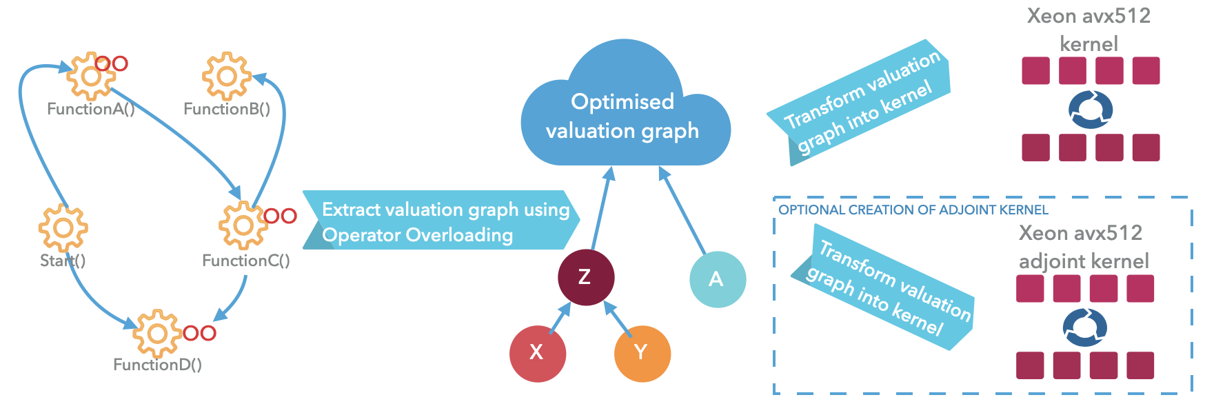
How AADC transforms code into optimized kernels
Code Generation AAD™ uses operator overloading to trace the exact sequence of operations performed by your object-oriented code (C++, C#, or Python) at runtime, extracting a computational graph (DAG). This DAG is then compiled to optimized machine code kernels. AADC is not a source code compiler—it preserves your coding style and abstractions while eliminating their runtime penalties, delivering native performance on standard CPUs with minimal code changes (replacing double with idouble in hot sections).
The generated kernels are reusable for repeated executions (e.g., thousands or millions of simulation paths, scenarios, or model calibrations), achieving 6–1000× speedups for both forward evaluations and first- or higher-order derivatives.
Designed for cross-platform execution, Code Generation AAD™ works across scientific simulations (PDEs, geophysics), quantitative finance, machine learning workflows (time series, recurrent networks), and other domains requiring repetitive high-performance computation.
Kernel creation time is pivotal, as it forms part of overall execution. Using off-the-shelf compilers (e.g., LLVM or C++) can take time equivalent to over 10,000 executions of the original code, making it prohibitive for smaller or dynamic simulations. This renders traditional code generation sufficient for testing but impractical for production, where minimizing compilation overhead is essential.
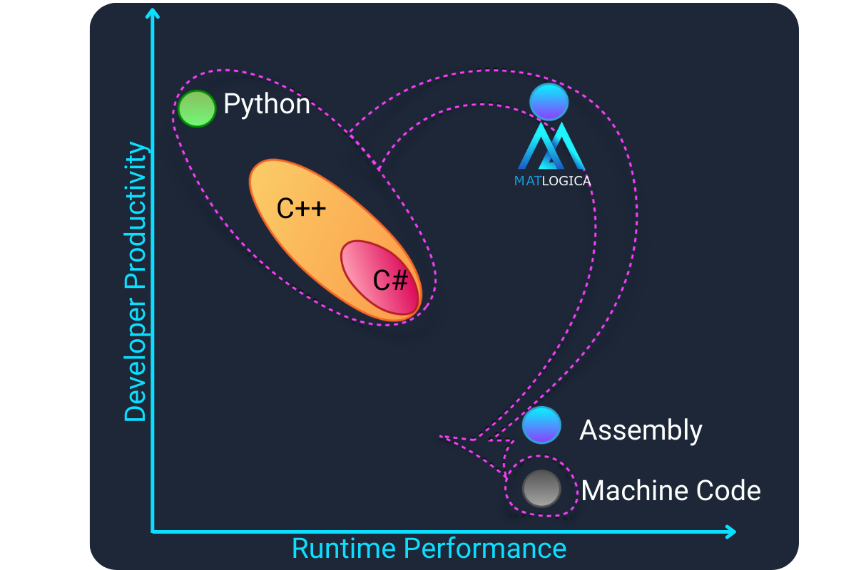
Traditional high-performance computing often forces a difficult trade-off: write in productive, high-level object-oriented languages (Python, C++, C#) and accept runtime overhead, or drop to low-level assembly/machine code for maximum speed — sacrificing readability and development velocity.
Fast compilation speed enables practical performance gains in production systems.
Avoids slow off-the-shelf tools, ensuring reliable integration across platforms.
How AADC transforms your code into optimized kernels
Regular program execution with I/O, setup, and data loading
Load data, read configuration, initialize objects
File reading, network calls, database queries
Any operations outside the hot computational section
Timing: Use native double (no overhead) or idouble (~2% overhead) for zero-cost transition to Phase 1
Capture hot section and generate optimized machine code
Replace double with idouble. Outside of recording, idouble has ~2% overhead vs native double.
Sequence of elementary operations automatically captured into DAG
Forward and adjoint passes generated in parallel; adjoint machine code generated backwards
Constant folding, dead code elimination, optimal register allocation
Timing: Recording/compilation adds overhead compared to a single execution. One-time cost amortized over kernel executions.
Multi-threaded execution even if original code isn't thread-safe
Run kernels across multiple threads even if original code isn't thread-safe
Single kernel execution returns value and all first-order sensitivities
Bump-and-revalue (finite difference) of first-order derivatives provides best results
Kernels are serializable - deploy to cloud for elastic compute without exposing source code
Performance: 6-1000x faster than original code, with adjoint factor <1
Reuse kernels for real-time and remote computation services
Save compiled kernels to disk for later reuse without recompilation
Kernels are compatible between Windows and Linux
Deploy kernels for always-on computation and real-time processing
Distribute kernels to remote compute nodes without exposing source code
Timing: Optional phase for production deployment scenarios
Not just AAD—all calculations benefit from JIT compilation
AVX2/AVX512 SIMD processes 4-8 doubles per CPU cycle. What would require manual assembly coding happens automatically.
Multi-threaded execution even if original code isn't thread-safe. Scales linearly with cores.
Optimal memory layout for modern CPU architecture. Data arranged for maximum cache efficiency and minimal bandwidth.
Better instruction cache usage through optimized code generation. Eliminates object-oriented overhead like virtual functions.
Python code compiled to native machine code, bypassing the interpreter entirely. Makes Python production-ready.
No virtual functions, no pointer chasing, no abstraction layers. Direct machine code for maximum performance.
What makes AADC uniquely powerful
AADC achieves the remarkable result where computing value AND all first-order sensitivities is faster than original code computing just the value—breaking the theoretical 'primal barrier'.
Traditional AAD has adjoint factor 2-5x. AADC achieves <1x relative to original code.
20-50x speedup when running multiple scenarios through the same kernel.
While AAD fundamentally reduces sensitivity computation from O(n) bumps to O(1) adjoint pass, AADC's JIT compilation, vectorization, and multi-threading optimizations make the combined value+sensitivities calculation faster than the original interpreted value-only calculation.
AADC delivers speedups ranging from 6× to over 1000× depending on your specific situation. The actual performance gain depends on several factors:
High-level implementations see the largest gains; already low-level optimized code sees smaller but still significant improvements
Python code typically sees larger speedups than C++ due to interpreter overhead elimination
Code without vectorization or multithreading benefits more from AADC's automatic optimizations
Complex models with many operations benefit from kernel compilation and memory optimization
Scenarios run many times (Monte Carlo, batch evaluation) amortize recording overhead for maximum gains
More sensitivities = larger advantage from AAD's O(1) adjoint pass vs O(n) bump-and-recompute
Contact us for a benchmark with your specific code to understand your expected performance improvement.
Complete API reference, integration guides, and code examples
Code Generation AAD™ — from first publication to industry recognition
"AAD: Breaking the Primal Barrier" published in Wilmott Magazine by Goloubentsev & Lakshtanov. First description of record-once replay-many, JIT-compiled adjoint kernels, and adjoint factor <1.
"Remarks on Stochastic AAD and Financial Models Calibration" published on arXiv, extending Code Generation AAD to calibration problems.
"A New Approach to Parallel Computing Using AD" published in Intel Parallel Universe Magazine.
"Automatic IFT" published in Risk.NET — #1 most-read for over a quarter.
Banking Tech Awards: FinTech Start-up of the Year. Accenture FinTech Innovation Lab Graduate. Chartis STORM50 #10.
Asia Risk Technology Awards: Technology Newcomer of the Year. Chartis Quantitative Analytics 50: Category Leader in Automatic Differentiation.
Intel publishes developer article on AADC's record-once replay-many paradigm for Python and C++ analytics.
Chartis Quantitative Analytics 50: Category Leader (consecutive years). EuroCC Supercomputing Accelerator Company.
Now that you understand how it works, explore what you can build with it