

The insurance industry burns hundreds of compute-hours on a problem with a known mathematical solution. Banks solved it over a decade ago. Insurance hasn’t. I wanted to understand why, and whether the barriers were real or just inertia.
The problem: bump-and-revalue
Every life insurer, pension fund, and annuity provider must answer the same question: how sensitive is our portfolio to market movements?
How much does the value change when rates move 1bp? When equity volatility rises 1%? When credit spreads widen?
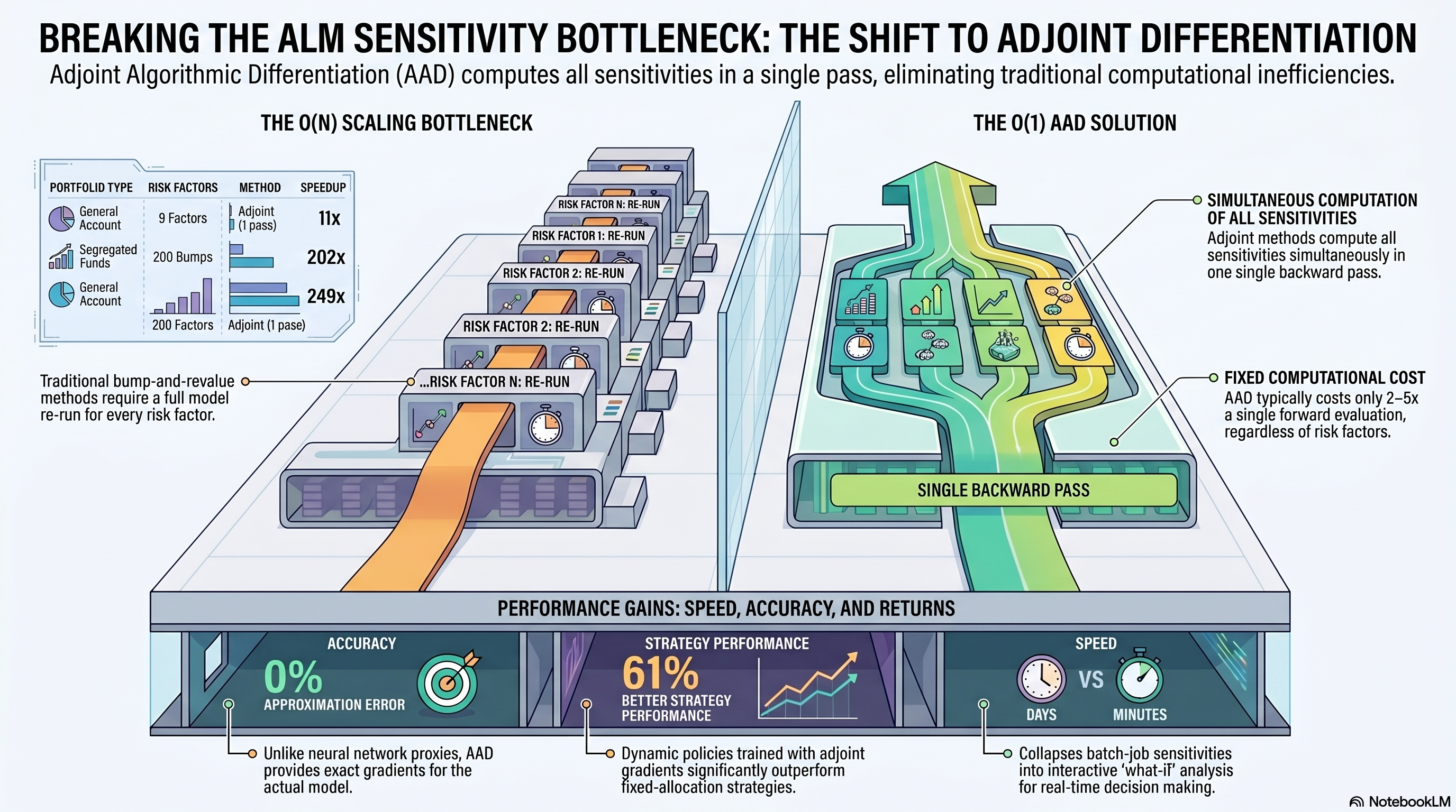
The standard method is bump-and-revalue. Change one parameter. Re-run the entire model. Record the difference. Do this for every risk factor.
A typical insurer has 50 to 200 risk factors. That means 100 to 400 full model re-runs. If each takes an hour, you’re looking at days of compute for sensitivities alone.
Aon’s PathWise platform uses GPUs to make each run faster. Their January 2025 whitepaper reports a 1,500× speedup per run. That’s real. But for 240 sensitivity scenarios (their M&A case study), it still takes 34 minutes of GPU time. Faster bumping is still bumping. Conning won ALM Solution of the Year in 2024 partly for using neural networks to approximate liability models. Faster, yes, but you’re differentiating an approximation, not the actual model. The industry knows the computation problem exists. So far the response has been faster hardware or cheaper approximations.
Banks solved this. Insurance didn’t.
Adjoint Algorithmic Differentiation (AAD) computes all sensitivities in a single backward pass, regardless of how many risk factors you have.
One forward pass gives you the portfolio value. One reverse pass gives you every sensitivity simultaneously. Cost: roughly 2–5× a single forward evaluation. Not .
Capriotti and Giles surveyed this in “15 Years of AAD in Finance” (Quantitative Finance, 2024). The paper covers CVA, XVA, SIMM, market risk. Banks have been doing this since the early 2010s.
Insurance? Not mentioned once. We checked. We went through Anna’s Archive, arXiv, SSRN, Google Scholar, and every major vendor’s published materials. Schlögl (2022) tried operator-overloading AAD for a simplified Solvency II model but hit a tape memory wall at 120-month simulations. Cathcart et al. (2023) applied forward-mode AD to actuarial models but noted that reverse mode was “prohibitive.” As far as we can tell, nobody has published a working reverse-mode implementation for insurance ALM.
Why insurance hasn’t adopted it
I keep hearing “AD doesn’t work for insurance.” That’s wrong. The barriers are engineering, not math.
AXIS, Prophet, RiskAgility all use proprietary scripting languages that AD tools can’t instrument. Banks write pricing libraries in C++, which AD tools handle fine. Right there, that locks out the entire installed base.
Then there are the discontinuities. A 30-year insurance simulation has hundreds of if/else branches for mortality, lapses, guarantee triggers. AD needs differentiable operations. You have to smooth these out, which takes care but isn’t the dead end people assume it is.
Nested simulation is the one that scared people most. Solvency II capital requires simulation-within-simulation. Differentiating through that looked intractable. It took rethinking, but it works.
There’s also an education gap that nobody talks about. The SOA and IFoA curricula cover statistics and demographics, not numerical methods. 80% of actuaries cite time as their main barrier to learning new technology. AD isn’t on their radar. Nobody put it there.
And nobody built the optimization loop. Even with sensitivities, most ALM is still manual. Pick an allocation. Run scenarios. Stare at the distribution. Adjust. Repeat. The step from “here are your sensitivities” to “here is a better allocation” was missing.
None of these turned out to be showstoppers.
What we measured
We built three proof-of-concept models. Everything below ran on the same machine (8 CPU threads, no GPU), and every number is from an actual run.
100-position general account portfolio
A general account with 40 government bonds, 30 investment-grade corporates, 15 high-yield, 10 mortgage pools, and 5 equity positions. $1.1 billion total, weighted duration 7.7 years.
Nine risk factors on the tape: rate curve at 4 tenors (2Y, 5Y, 10Y, 30Y), IG and HY credit spreads, equity level, equity volatility, mortgage prepayment rate.
| Method | Time | Sensitivities | Speedup |
|---|---|---|---|
| Forward only | 29 ms | 0 | — |
| Adjoint (1 pass) | 41 ms | All 9 | 11× |
| Bump-and-revalue | 453 ms | 9 | — |
At 100 factors, the speedup reaches 125×. At 200, it’s 249×.
30-policy segregated fund portfolio
10 GMDB, 10 GMWB, 10 GMAB. Each policy has its own age, premium, and contract features. Stochastic interest rates (Hull-White, correlated with equity). 45-year projection horizon.
All 30 policies sit on a single computation tape. One reverse pass produces delta, vega, and rho for the entire portfolio.
| Method | Time | Sensitivities | Speedup |
|---|---|---|---|
| Forward only | 1,746 ms | 0 | — |
| Adjoint (1 pass) | 3,467 ms | All 3 | — |
| B&R (50 bumps) | 88 sec | 50 | 51× vs adjoint |
| B&R (200 bumps) | 350 sec | 200 | 202× vs adjoint |
The 200-factor number is the one I’d pay attention to. Most seg fund programs don’t hedge gamma because second-order sensitivities cost too much with bump-and-revalue. With adjoint, it becomes a rounding error on top of the base evaluation.
Optimal dynamic asset allocation
A CalPERS-like pension fund (79% funded, the hard case) allocating across government bonds, corporate bonds, and equities over 10 years. A neural network learns the best allocation by gradient ascent, using exact adjoint gradients through the full 120-month stochastic simulation.
Training takes about 2.5 minutes. 1,500 iterations on 2,048 scenarios, with fresh random paths every 50 iterations to prevent overfitting.
| Strategy | Objective |
|---|---|
| All bonds (0/0/100) | 5.56 |
| Conservative (20/15/65) | 11.19 |
| Balanced (35/20/45) | 14.71 |
| Aggressive (50/25/25) | 16.41 |
| Learned (dynamic) | 26.40 |
The learned policy beats the best fixed strategy by 61%. A fixed allocation can’t respond to a rate drop or a funding ratio dip. The learned one does, and the adjoint gives it the exact gradient signal to figure out how.
What the academics tried instead
Krah et al. (2020) trained neural networks to approximate the model output, then used the approximation instead of the real thing:
| Method | VaR Error | ES Error |
|---|---|---|
| Polynomial proxy | 3.6% | 3.0% |
| Neural network proxy | 1.1% | 0.4% |
| Adjoint (exact model) | 0.0% | 0.0% |
Proxy models exist because each full model evaluation is supposed to be expensive. Ours takes 18 milliseconds. When the real thing is that fast, why bother with an approximation?
What this is and what it isn’t
As far as we can find, this is the first working application of reverse-mode adjoint AD to insurance ALM. We searched systematically across academic databases, vendor publications, and conference proceedings.
It is not a production system. These are simplified models. They don’t have IFRS 17 CSM accounting, full Solvency II or LICAT compliance, or the regulatory audit trails that AXIS and Prophet provide. We’re not claiming to replace those platforms. This is a computation engine that would sit alongside them.
I want to be clear about the Aon comparison. Aon processes 100K policies on GPUs. Our benchmark has 100 positions on CPUs. The per-unit throughput isn’t comparable, and I’m not pretending it is. What we bring is different: the adjoint eliminates of reruns. That advantage holds regardless of what hardware you run on.
What this means in practice
The sensitivity bottleneck in insurance isn’t a hardware problem. GPUs make each bump faster, and that helps. But bump-and-revalue scales as , and adjoint stays at . No amount of hardware closes that gap.
For an insurer bumping 50 to 200 risk factors, adjoint collapses that to one reverse pass. You stop computing sensitivities as a batch job and start computing them while people are still in the room making decisions.
Gamma hedging for seg fund portfolios becomes affordable. What-if analysis gets fast enough to actually be interactive. Solvency monitoring doesn’t have to wait for the quarterly run. None of that is speculative. It follows directly from sensitivities not costing anymore.
The math has been around for 15 years. The engineering turned out to be harder than the math, which is probably why it took this long. We have working demos if you want to see the numbers.
Benchmarks reproducible from source. Implemented using AADC, a commercial adjoint AD compiler (matlogica.com).