

Follow-up to Post 3: “What AAD-native architecture actually looks like”
Post 3 described four abstractions and three kernels. Pricing, Greeks, XVA, FRTB, SIMM all fall out of the same record-once, adjoint-once architecture. But I left out the fifth abstraction.
It’s the one worth paying attention to.
The fifth abstraction: decisions
Some products have decisions embedded in them. A Bermudan swaption exercises or doesn’t. A gas storage facility injects or withdraws. A policyholder surrenders or stays. A convertible bond converts or waits.
Traditional approaches treat these as separate problems. Longstaff-Schwartz regresses continuation values. Dynamic programming discretises the state space. Reinforcement learning samples random perturbations to estimate gradients. Each method has its own code, its own assumptions, and its own failure modes.
We treat decisions as an observable. At each timestep, a neural network takes the current state (fill level, spot price, time remaining, forward curve shape) and outputs a decision. Inject this much. Withdraw that much. Exercise now. The network’s weights sit on the computation tape alongside the simulation, the trade state, and the cashflow accumulation.
One reverse pass gives you the exact gradient of the objective with respect to every decision weight, computed through the entire simulation, every timestep, every constraint.
Why this matters
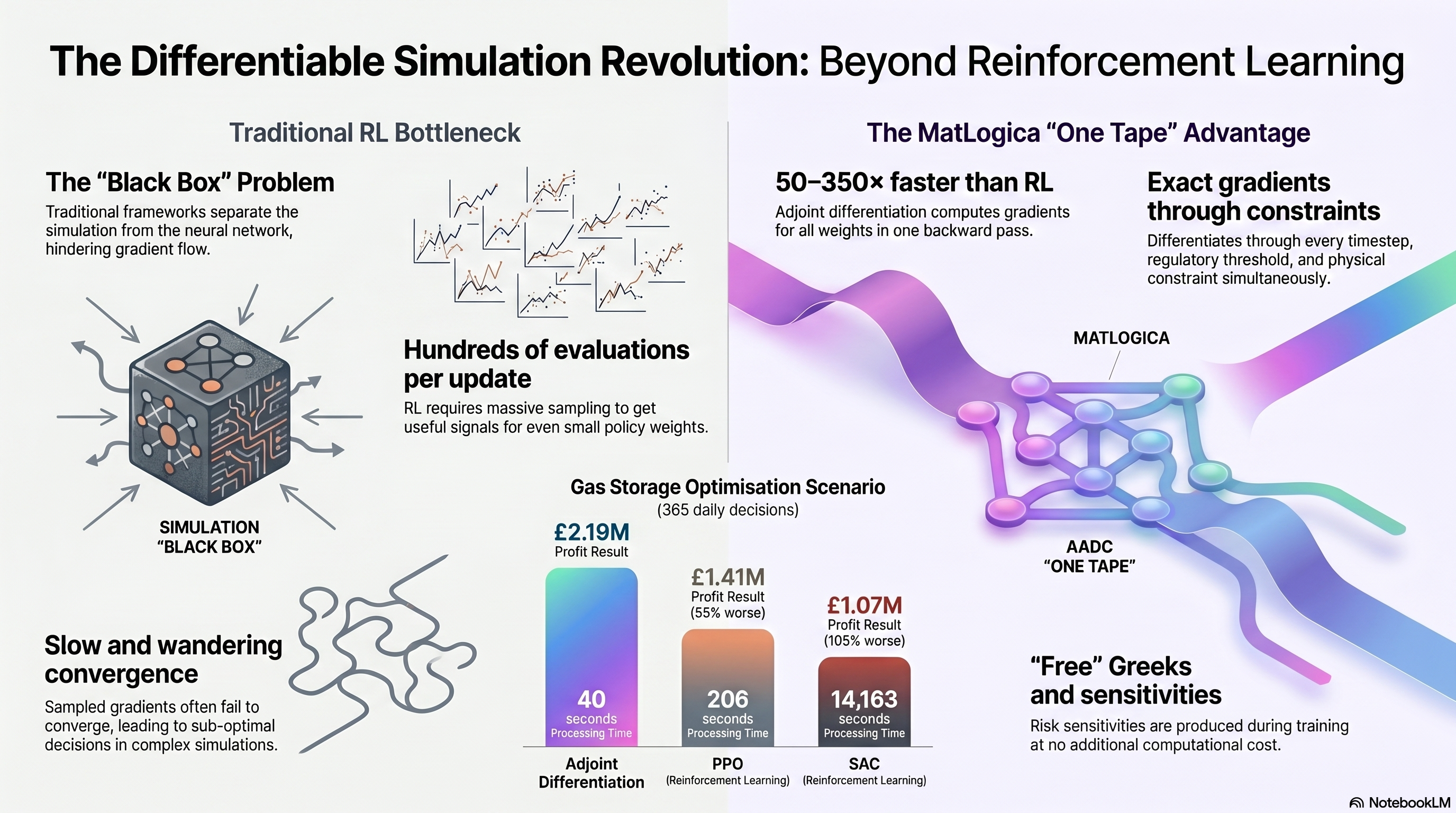
Reinforcement learning estimates gradients by running the simulation thousands of times with random perturbations and averaging. If you have 800 policy weights, each gradient estimate requires hundreds of random-direction evaluations to get a useful signal. Convergence is slow.
Adjoint differentiation computes the gradient of all 800 weights in one backward pass. Same cost as a single forward evaluation, roughly. The training loop becomes: forward pass (evaluate profit on a batch of paths), backward pass (exact gradient of profit with respect to every weight), Adam step. Repeat.
The numbers from gas storage, 365 daily decisions, 807 policy weights, measured on a single machine (Linux, Intel Xeon, 8 threads, no GPU):
| Method | Training Time | Value Achieved | vs Adjoint |
|---|---|---|---|
| Adjoint differentiation | 40 s | $2.19M | — |
| PPO | 206 s | $1.41M | 55% worse |
| SAC | 14,163 s (4 hrs) | $1.07M | 105% worse |
| REINFORCE | 10,000+ iterations | — | Did not converge |
What gets recorded
Everything. The stochastic price model (Schwartz-Smith two-factor, OU mean-reversion, whatever your quants specify). The neural policy evaluation at each timestep. The smooth constraint enforcement: capacity limits, rate limits, regulatory thresholds. The cashflow accumulation and discounting. The terminal penalties.
All of it flows through the active type. All of it lands on the tape. The reverse pass differentiates through the entire chain: flows backward through 365 days of cashflows, through 365 constraint projections, through 365 neural network evaluations, through 365 price model steps.
Standard deep learning frameworks cannot do this for this class of problem. They differentiate through the neural network, but the simulation (the price model, the physical constraints, the state evolution) sits outside the computation graph. They treat it as a black box and estimate gradients by perturbation. Differentiable simulation puts the box on the tape and differentiates through it.
The products
Variable annuity. GMDB guarantee, 35-year monthly projection, 100,000 paths. The policyholder’s surrender decision is a neural policy trained on the tape. Records in 187 milliseconds. Prices in 1.5 seconds. Full Greeks, through the mortality model, through the surrender policy, through 420 monthly timesteps, in 2.7 seconds.
Gas storage. Neural optimal control over a 365-day contract, 10,000 paths. The kernel is 637 KB of compiled forward code and 1.5 MB reverse. Records in 391 milliseconds. Prices in 721 milliseconds. Greeks through the entire neural policy in 1.4 seconds. Every forward curve delta, every vol sensitivity, computed through 365 daily exercise decisions.
The Greeks are free. Not “cheap.” Free. The same backward pass that trains the policy also produces , , , at every tenor. You don’t choose between training and risk. Both come from the same computation.
Beyond finance
The pattern (simulation plus neural policy plus constraints plus objective, all on one differentiable tape) is not specific to finance.
| Component | Gas Storage | Battery Storage | Boiler NOx Control |
|---|---|---|---|
| Forward model | Schwartz-Smith 2F prices | GBM electricity + OU reserve | Combustion dynamics (Zeldovich NOx) |
| State | Inventory level | State of charge | 12-month rolling NOx average |
| Policy network | MLP 6→5→5→2 | MLP 7→5→5→2 | MLP 8→8→8→3 |
| Constraints | Capacity, injection/withdrawal rates | SoC limits, charge/discharge rates | Operating flow limits |
| Objective | Maximize cashflow | Maximize arbitrage profit | Maximize throughput, minimize fines |
An oil refinery faces regulatory fines when its 12-month rolling average NOx exceeds 0.07 PPM. We trained an optimal control policy in 26 seconds. Zero exceedance days versus 326 with the unoptimized policy. Free sensitivities: tells the operator exactly what looser regulation is worth.
The same pattern applies to battery storage dispatch, HVAC optimal control, robotic trajectory optimisation, any sequential decision problem where you can write down the dynamics and the objective.
The tradeoff, revisited
Post 3’s tradeoff was: every computation must flow through the active type. For pricing and Greeks, that’s a type-system constraint.
For neural optimal control, the tradeoff is sharper: the simulation itself must be differentiable. Hard if/else branches that depend on active variables bake one branch at recording time. You need smooth approximations (we use a rational sigmoid that’s cheaper than exp and never overflows) or a branch manager that records both branches and selects per scenario at evaluation time.
In practice this is not a real limitation. Smooth constraints are standard in optimal control theory. The rational sigmoid converges to the hard step as sharpness increases. And you get exact gradients through the entire computation, simulation, policy, constraints, objective, in a single pass.
What this means
If you have a sequential decision problem (exercise, storage, dispatch, control) and you’re solving it with RL, dynamic programming, or Longstaff-Schwartz, you have an alternative. Record the simulation on a differentiable tape. Put a neural policy on the same tape. Train with exact gradients. Deploy the trained weights.
The training is 50 to 350 times faster than RL. The result is better because exact gradients converge where sampled gradients wander. The Greeks are free. And the architecture is the same one that prices your vanilla book and computes your FRTB sensitivities.
One tape. Forward pass for the price. Backward pass for everything else.
Implemented using AADC, a commercial adjoint AD compiler (matlogica.com). The differentiable simulation patterns described here require a tape-based AD system that supports control flow recording, kernel compilation, and SIMD evaluation.